BioInfoSummer2015 SLiMSuite Workshop

Dr Richard Edwards, University of New South Wales
Thursday 10^th December 2015

Session outline

Click for slides.

Part I: Theory

• Introduction to workshop
• What are SLiMs?
• What is SLiMSuite

Part II: Practice

• Installing/running SLiMSuite
• Data types and main input formats
• Motif discovery using the SLiMSuite REST Servers
• Motif discovery using the SLiMScape app for Cytoscape

Additional help and documentation

General information about SLiMs and motif discovery can be found in the literature. Some good places to start are the recent ELM 2016 paper and our 2015 Methods in Molecular Biology review as well as the SLiMScape app paper:

• Motif discovery review paper (PDF)
• SLiMScape app paper (PDF)
• SLiMFinder manual (PDF)
• SLiMProb manual (PDF)
• CompariMotif manual (PDF)

For information about SLiMSuite, please visit the EdwardsLab webpage and the SLiMSuite blog. Help and documentation for the REST servers can also be found at the REST homepage. If in doubt, please email: richard.edwards@unsw.edu.au.

Several EdwardsLab publications also cover motifs and SLiMSuite tools.

Installing/Running SLiMSuite

NOTE: For this workshop, you do not need to install SLiMSuite. You will need Cytoscape and the SLiMScape app for the later parts.

---

The current SLiMSuite release is 2015-11-30 and can be downloaded by clicking the button (left).

In addition to the tarball available via the links above, SLiMSuite is now available as a GitHub repository (right).

See also: Installation and Setup.

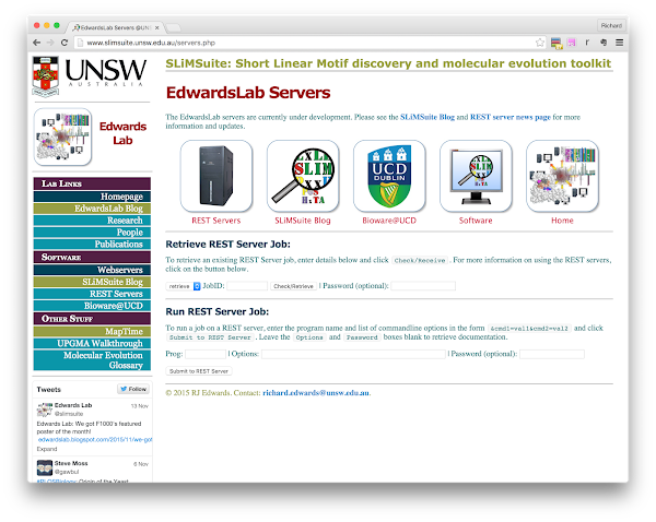
For this workshop, we will primarily be running the tools (and looking at pre-generated results) via the online servers:

Data types and main input formats

From a computer science perspective, input and output for SLiMSuite is just plain ASCII text. This makes it easy to plug SLiMSuite into existing scripts and pipelines - and manually view/edit any input or output files if required. However, “plain text” is not very informative, and SLiMSuite actually deals with a lot of different formats of plain text (from a “human formatting” rather than “file type” point of view). The documentation is currently in the process of being updated to better reflect these formats but some commandline options will still simply list FILE, FILES or FILELIST as input parameters: see the accompanying descriptions to see what format these should be. Ask if it’s not clear! (File format documentation will also be added to the SLiMSuite blog, so check there.)

Within SLiMSuite, each file type has a distinct “file extension” that denotes the file type. Note that these are not enforced for input, although some programs may not always recognise the right format if a different extension is used. If you get odd input behaviour/errors that you do not understand, see if changing the file extensions helps. If you want a common file extension to be auto-recognised, let me know and I might be able to add it. SLiMSuite file extensions will not necessarily be recognised by other programs. NOTE: Operating systems will sometimes hide file extensions by default. If you are getting very confused, or have problems of extra *.txt extensions on everything, try changing the system settings. (And/or becoming familiar with command-line file manipulation.)

The main input formats for SLiM discovery are:

• A source of protein sequence data. This could be a protein FASTA file, a Uniprot plain text file, or a list of Uniprot accession numbers to download. For some tools, a single Uniprot accession number will work.
• A source of motif (regular expression) definitions. This is only required if looking for known (or other pre-defined) motifs and/or wanting to compare a set of de novo predictions with known motifs. A number of different formats are accepted for motif input, including SLiMFinder (summary) results and ELM downloads. The simplest/easiest is a plain text file of regular expressions. For more on motif regular expression formats, please see Edwards and Palopoli 2015.

Common motif discovery tasks

Jobs can be run and retrieved at: http://www.slimsuite.unsw.edu.au/servers.php. (This is a bit easier than making the URL directly, although this is also an option as we will see.)

NOTE: Some of the jobs take a while to run and the SLiMSuite servers have limited resources. It would therefore be useful if you could click on the example JobID links rather than trying to run every example REST command yourself. The first output tab (and the log tab) will show you the run times for that job, so you can see which jobs are fast or slow before you experiment.

---

Task 1: Find known SLiMs in a protein (ELM/SLiMProb)

ELM. Visit http://http://www.elm.eu.org/ and enter your protein of choice as Uniprot identifier or accession number in the box. (Identifiers will auto-complete and fill in some extra details.) For non-Uniprot protein sequences, you can also enter fasta format.

Try this now with P03070 (LT_SV40) or P03254 (E1A_ADE02). Each of them should have a True Positive LIG_Rb_LxCxE_1 motif.

SLiMProb. We can do a similar search using the SLiMProb REST server (paste the contents of the grey box onto the end of the http://rest.slimsuite.unsw.edu.au/ URL):

slimprob&uniprotid=E1A_ADE02&motifs=elm

JobID: 15120800029

NOTE: The ELM alias currently searches the 2015 ELM classes.

---

Task 2: Find custom SLiMS in a protein (SLiMProb)

slimprob&uniprotid=E1A_ADE02&motifs=LxCxE,PxDLS

JobID: 15120800031

---

Task 3: Finding proteome-wide occurrence of a motif using Bioware (SLiMSearch)

The SLiMSearch server is accessible at: http://slim.ucd.ie/slimsearch/. This has been recently updated to Version 4 and now brings in a lot of information, so it is recommended that you read the Help pages for the server.

Example (LIG_CtBP_PxDLS_1): http://slim.ucd.ie/rest/#/slimsearch/annotations?jobId=7R8Tvssm9HEdjWW7jQsgEHUfP0VlHdR6

Human protein PRDM16 is particularly interesting: it does not have an annotated ELM but does match a region annotated to interact with CTBP1. (See the Region column - Expand the instance Feature annotations for a clearer look.) This kind of search can be a good way of identifying new instances of known motifs - some of which may be in the literature but may not have yet made it into database annotation.

The ELM definition for this motif P[LVIPME][DENS][LM][VASTRG] is very degenerate with a lot of hits - over-prediction is a big problem in motif discovery. We can try to make the definition a little tighter as the expense of some instances, using another tool called SLiMMaker:

slimmaker&peptides=LIG_CtBP_PxDLS_1&iterate=T&align=F&minfreq=0.67&minseq=2

JobID: 15120600004

Repeating the SLiMSearch analysis with the redefined motif (P[EILMV][DN]L[ARST]) gives a greater density of known ELMs (see the Motif column) in the top ranked motifs: http://slim.ucd.ie/rest/#/slimsearch/annotations?jobId=L41BRpXQ1oTD6ByDuUSqjWbQZ22WBKbw.

---

Task 4: Predicting novel SLiMs de novo in a set of proteins (SLiMFinder)

SLiMFinder is designed to look for convergently evolved motifs that are shared between unrelated proteins. For example, we can look at the proteins known (in ELM) to contain the LIG_PCNA_PIPBox_1. As SLiMs are generally in disordered regions, we will switch disorder masking on with dismask=T, which uses IUPred to predict globular regions, which are masked out:

slimfinder&uniprotid=LIG_PCNA_PIPBox_1&dismask=T

JobID: 15120800001

(We will look at the UPC and motif cloud output among others.)

---

Task 5: Identifying known motifs from de novo predictions (CompariMotif)

When you have a lot of motif predictions, it can be tiresome and error-prone to manually scan them for things that look familiar. SLiMSuite has a tool called CompariMotif, which compares sets of motifs for similarity.

The comparimotif server can take motif files/lists (like SLiMProb or SLiMFinder output directly. These are given to the &motifs and/or &searchdb options: if no &searchdb is given then the input motifs are searched against themselves. (This can be useful if clouding goes a bit wrong.)

To pass the output of one server to another, use the format: &cmd=jobid:XXXXXX:OUTFMT, where XXXXXX is the Job ID and OUTFMT is the desired output format. E.g.:

comparimotif&motifs=jobid:15120800001:main&searchdb=LIG_PCNA_PIPBox_1

JobID: 15120900004

The server is currently in development so output is not sorted usefully yet. This is more of a problem if searching against many SLiMs:

comparimotif&motifs=jobid:15120800001:main&searchdb=elm

JobID: 15120900005

The best advice is to save the compare output table (retrieve&jobid=15120900005&outfmt=compare), open it up in Excel and sort on Score. Alternatively, use the CompariMotif server at http://bioware.ucd.ie.

---

Task 6: SLiM prediction with conservation masking (SLiMFinder)

Masking is important as it reduces the search space. It can also reduce the signal if it incorrectly masks some true positives but for larger datasets the reduction in "noise" can be more important. As well as dismask=T/F there are several other masking options in SLiMSuite:

• low complexity masking (ON by default)
• N-terminal methionines (ON by default)
• conservation-based masking (OFF by default)
• Uniprot feature masking (OFF by default)
• Motif masking (OFF by default)

For custom sequence input, there is also the option for custom masking based on upper/lower case. For now, we will just look at conservation masking, as this has been shown to improve sensitivity in PPI data. For example, a 2013 compilation of CTBP1 interactors does not yield a significant motif:

slimfinder&uniprotid=CTBP1&dismask=T&runid=CtBP1-DisMask

JobID: 15120900002

But if consmask=T is also switched on:

slimfinder&uniprotid=CTBP1&dismask=T&consmask=T&runid=CtBP1-ConsMask

JobID: 15120900003

The importance of correcting for evolutionary relationships

The UPC correction can be switched off with efilter=F. Many motif prediction tools calculate estimated expectations without such correction. This can result is massive biases due to shared evolutionary history, which swamp any convergent SLiM evolution signal, for example with the LIG_CtBP_PxDLS_1 ELM proteins:

slimfinder&uniprotid=LIG_CtBP_PxDLS_1&dismask=T&runid=CtBP-NoEFilter&efilter=F

JobID: 15120800036

---

Task 7: Look for enrichment or depletion of motifs in a set of proteins (SLiMProb)

We can investigate why the PxDLS motif did not come back with just disorder masking by looking at its enrichment using SLiMProb. When given multiple proteins, SLiMProb will use the same UPC correction as SLiMFinder but also return statistics without UPC correction and simply treating all the sequences as one giant sequence. It can, for example, be used to investigate different definitions of a motif:

slimprob&uniprotid=CTBP1&dismask=T&runid=CtBP1-DisMask&motifs=PxDLS,P[LVIPME][DENS][LM][VASTRG],Px[DE][LM][ST]

JobID: 15120900016

In this case, we can see that even though the "true" motif has the most support, it is also expected to occur more by chance. It is enriched, but not enough to survive the multiple testing correction of SLiMChance.

Though not of interest here, the pUnd statistics can be used to look for depletion/avoidance of a particular motif in a dataset.

---

Task 8: Find novel motifs from a conservation pattern (SLiMPrints)

Patterns of evolutionary conservation can also be used to directly identify regions of proteins that look like motifs. The tool we have developed for this is called SLiMPrints, which can be run at the Bioware SLiMPrints server. For example, we can look for motif-like regions in one of the CtBP PPI partners, FOG1_HUMAN (Q8IX07): http://bioware.ucd.ie/~compass/biowareweb/cgi-bin/PHP_helper_files/slimprintsInfo.php?jobId=e7GZLf

This protein has a bunch of significant motif-like regions, including the PxDLS motif region at rank 7: http://bioware.ucd.ie/~proviz/ProViz/alignmentViewer/drawer.php?uniprotid=Q8IX07&slim=GPIDL&slimpos=793&column=794.5&width=80&collapse=false

(Note how the precise motif is rarely returned by de novo predictors.)

---

Task 9: Using the SLiMScape app to visualise a server job

We're now going to fire up Cytoscape and have a quick look at the SLiMScape app. This is fairly well described in the paper, so we will just look at the main ways to run the server. If you've not used Cytoscape before, you'll want to visit the Cytoscape website and watch the introduction video, before installing it.

The simplest is to retrieve an existing run:

1. In the SLiMFinder tab, enter 15120900003 in the Run ID box and hit Retrieve.
2. Apply the default layout.
3. Explore the results. Connections are UPC relationships in the data.

---

Task 10: Running QSLiMFinder through SLiMScape

Now let's imagine we had seen the SLiMPrints results from above for FOG1_HUMAN and knew that it interacted with CtBP1. We could ask the specific question if any motifs in FOG1_HUMAN were enriched in the rest of the PPI dataset. We do this by using QSLiMFinder and giving Q8IX07 as the query. (&query=Q8IX07 on the server.)

First, add a node to the network and change its name to Q8IX07. Enter this in the Query Sequence box then highlight all of the nodes before hitting Run QSLiMFinder:

JobID: 15120900007

This is the essence of molecular mimicry and we could use the same approach to see if E1A_ADE02 shares any motifs by adding P03254 and using it as a query:

JobID: 15120900008

---

Task 11: Building PPI networks for analysis

The most useful thing of having access to SLiMSuite through Cytoscape is to be able to use it to explore PPI networks and select nodes for analysis. There are in-built tools to get PPI data into Cytoscape. For SLiMSuite, the ID must be a Uniprot ID or accession number, or a Node must have "Uniprot" attribute.

The SLiMSuite REST server also provides some methods for getting PPI data into Cytoscape (and/or for use on the server), using the PINGU server. This is still under development and so the documentation of the available PPI data is currently limited, but just get in touch if you want to use it. (Currently human only.)

PPI data is retrieved by entering one or more gene symbols as a &hublist, optionally along with a &ppisource (see the ppisource alias):

pingu&hublist=CTBP1,CTBP2&ppisource=intact

JobID: 15120900009

This can be used directly for &uniprotid input using the &rest=uniprot output:

slimfinder&uniprotid=jobid:15120900009:uniprot&dismask=T&consmask=T&runid=CtBP1and2

JobID: 15120900011

Alternatively, the PPI data can be imported into Cytoscape using the pairwise table:

1. Start a new session. (Later you can workout how to import and merge networks.)
2. Import network from URL: http://rest.slimsuite.unsw.edu.au/retrieve&jobid=15120900009&rest=pairwise
3. Rename the HubUni and SpokeUni fields to name and attribute them to Source Node and Target Node attributes. Make Hub the Source, Spoke the Target and Evidence the Interaction Type then import.
4. Select the nodes that are shared interactors of both CtBP proteins.
5. Modify the masking settings to include disorder, conservation and feature masking.
6. Hit Run:

JobID: 15120900013

New SLiMSuite REST Servers

Since the move to UNSW in 2013, the Bioware SLiMSuite servers and REST servers have been undergoing some much needed TLC. As part of this process, a new set of UNSW REST servers were introduced and online with the 2015-06-01 SLiMSuite release.

An overview of how the REST servers work is given on the REST Homepage. The available tools are listed at the REST Tools page. The main ones - accessible through the SLiMScape app for Cytoscape are (or support):

• SLiMFinder de novo SLiM discovery.
• QSLiMFinder query-focused de novo SLiM discovery.
• SLiMProb defined/known SLiM prediction.
• SLiMMaker Simple Regex SLiM generation from peptides.

The primary focus has been setting up new servers to be accessed via a RESTful-style interface whereby a URL can be directly given to the server and used to either download results directly (if accessing programmatically) or view in a web browser. As with the main programs, these servers use plain text inputs and outputs wherever. Whilst this probably makes proper computer scientists very unhappy, it should make it very easy to incorporate SLiMSuite REST functions into your own scripts - you only need to learn how to parse text. (It also makes it easy for me to swap input sources.) If you don’t want to write your own, SLiMParser is provided in the SLiMSuite download to do this for you.

The other design consideration that has gone into the REST servers is to make them run as much like the commandline versions as possible: (1) they use the same code; (2) they use the same commandline options, parsed from the URL. This means that (a) you should easily be able to reproduce server results on your own system, and (b) new functions (and bug fixes) should become quickly available via the REST servers.

To save the need for constructing complex URLs, there is a simple on-size-fits-all form at the EdwardsLab server page. Over time, tool-specific forms will be established. Currently, this only exists for SLiMMaker.

As ever, if something about the new servers misbehaves or does not make sense - or you really want some new functions - please get in touch.

SLiMSuite bug with combined sequence case and disorder masking

A small flaw has been discovered in the current implementation of disorder masking when it is combined with masking upper or lower case residues (casemask=X dismask=T). Rather than predicting disorder on the unmasked sequence and then combining with any case masking, disorder predictions are currently made on the masked sequences.

Hopefully, this will have minimal impact for the majority of cases. (Although I am not certain, I suspect that it will produce a tendency to over-predict disorder and thus under-mask.) This bug has been fixed for the next release of SLiMSuite. Note that other masking combinations are not affected.

New SLiMSuite release now available

A new download of SLiMSuite (release 2014-06-22) is now available.

As well as fixing the minor GOPHER output bug, a new Taxonomy processing module (rje_taxonomy) has been added. Although primarily designed for use with other SLiMSuite programs, this module has some standalone functionality for generating lists of Taxa IDs and species codes. (Details to follow.)

Output for the main SLiMSuite programs, SLiMFinder, SLiMProb and QSLiMFinder has also been consolidated and made more consistent for both re-running analyses and running analyses with multiple settings (consecutively) in the same directory. The use of GOPHER for generating alignments for conservation masking in these programs has also been improved to enable forking. (Details to follow.)

The final change of note is that SLiMMaker is now used to generate a consensus motif for each cloud returned by (Q)SLiMFinder. Note that (by default), these consensus motifs will not necessarily cover all occurrences in the cloud. (See SLiMMaker for more information.)

Other miscellaneous updates are listed below.

Updates since last release:

• gablam: Updated from Version 2.12.
→ Version 2.13: Fixed Protein vs DNA GABLAM. Modified sequence extraction to handle larger sequences. Add blastdir=PATH/.

• gopher: Updated from Version 3.3.
→ Version 3.4: Fixed FullRBH paralogue duplication issue.

• pingu_V4: Updated from Version 4.1.
→ Version 4.2: Bug fixes for use of PPISource to create PPI databases. Add HGNC to sourcedata (xrefdata=HGNC)

• qslimfinder: Updated from Version 1.7.
→ Version 1.8: Added cloudfix=T/F Restrict output to clouds with 1+ fixed motif (recommended) [False]. Consolidating output.

• slimbench: Updated from Version 2.2.
→ Version 2.2: Modified the FN/TN and ResNum calculations. No longer rate TP in random data as OT.
→ Version 2.3: Changed the default to queries=F. SearchINI bug fix. Added occbench generation.

• slimfarmer: Updated from Version 1.1.
→ Version 1.2: Implemented the slimsuite=T/F option and got SLiMFarmer qsub to work with GOPHER forking.

• slimfinder: Updated from Version 4.6.
→ Version 4.7: Added SLiMMaker generation to motif clouds. Added Q and Occ to Chance column.

• slimprob: Updated from Version 1.2.
→ Version 1.3: Consolidating output file naming for consistency across SLiMSuite. (SLiMBuild = Motif input)

• rje: Updated from Version 4.10.
→ Version 4.11: Enabled '\t#' comments in ini files. Modified getStrLC to return '' for 'none' by default. Added listMax().
→ Version 4.11: Added self.name() to basic object class.

• rje_blast: Reinstated for SLiMDisc legacy compatibility.

• rje_ensembl: Reinstated and updated.
→ Version 2.11: Added rje_taxonomy and makeuniprot=T/F. Removed metlist. Moved release and species data extraction.
→ Version 2.12: Changed chromspec to enable downloads of all species but also download toplevel files, not chromosomes.

• rje_hmm_V1: Reinstated.

• rje_hpc: Updated from Version 1.0.
→ Version 1.1: Disabled memory checking in Windows and OSX.

• rje_motif_V3: Updated from Version 3.0.
→ Version 3.1: Fixed minor code bugs.

• rje_obj: Updated from Version 1.6.
→ Version 1.7: Added self.name() to basic object class.

• rje_seq: Updated from Version 3.18.
→ Version 3.19: Fixed BLAST+ sequence extraction name truncation error.

• rje_seqlist: Updated from Version 1.4.
→ Version 1.5: Added sampler=N(,X) : Generate (X) file(s) sampling a random N sequences from input into seqout.N.X.fas [0]
→ Version 1.6: Modified currSeq() and nextSeq() slightly to fix index mode breakage. Look out for other programs breaking.
→ Version 1.6: Add sequence fragment extraction.

• rje_slim: Updated from Version 1.6.
→ Version 1.7: Fixed import slimFix(slim) error that was reporting slimProb()

• rje_slimcalc: Updated from Version 0.7.
→ Version 0.8: Made RLC the default.

• rje_slimcore: Updated from Version 1.14.
→ Version 1.15: Added pre-running GOPHER if no alndir and usegopher=T. Updated dataset() to use Input not Basefile.

• rje_taxonomy: Created/Renamed.
→ Version 0.0: Initial Compilation.
→ Version 0.1: Initial working version with rje_ensembl.
→ Version 1.0: Fully functional version with modified viral species code creation.

• rje_uniprot: Updated from Version 3.18.
→ Version 3.19: Updated and consolidated dbxref table generation (formerly linkout) using rje_db. Changed acc_num to accnum.

File management for large SLiMSuite runs

The latest release of SLiMSuite features a slight modification to the way that files are generated and tidied, which can be beneficial for large runs.

Previously, a different results directory (resdir=PATH) was required for each different run to avoid dataset-specific results being over-written. The partial exception was the *.pickle.gz file, which included some SLiMBuild information in its name. (This is predominantly to speed up the ability of (Q)SLiMFinder to recognise when an intermediate pickle file can be used or not.) As of the latest release, the RunID (runid=X) is also now included in dataset-specific output, allowing results from several different runs (with different RunIDs) to go into the same results directory.

The exception is the files that are created as part of the initial setup/SLiMBuild process: *.slimdb, *.dis.tdt and *.upc. From a given Dataset and RunID, the following files will therefore be generated in ResDir/

Dataset.RunID.cloud.txt
Dataset.RunID.mapping.fas
Dataset.RunID.maskaln.fas
Dataset.RunID.masked.fas
Dataset.RunID.motifaln.fas
Dataset.RunID.occ.csv
Dataset.dis.tdt
Dataset.#SLiMBuild-Text#.pickle.gz
Dataset.slimdb
Dataset.upc

Note that the default ResDir is SLiMFinder/, QSLiMFinder/ or SLiMProb and the default RunID is the date and time of the run.

TarGZ and SaveSpace

Obviously, the results directory can quickly fill up with files if there are multiple datasets and/or runs with different RunIDs. The way to get round this is to use the targz=T and savespace=X options.

targz=T will package up all of the files associated with a specific run into a single Dataset.RunID.tgz file. This does not work on Windows. (Note that previous versions generated a Dataset.tar.gz file.) The *.pickle.gz file associated with the run will not be included in the tar file unless savespace=2+ (see below).

Note: the tar file is actually generated from the run directory, not the results directory and will include the relative path to ResDir in the tarred files. This means that if you enter ResDir/ and then tar -xzf Dataset.RunID.tgz, an additional ResDir/ will be created in which the files can be found. This is actually pretty useful as it allows the user to unpack individual runs and then delete the whole directory when finished. To return individual results to their “rightful” place, simply run the tar command from the same directory that the SLiMSuite program was run from (e.g. tar -xzf ResDir/Dataset.RunID.tgz).

The savespace=X option saves space by deleting excess files. It is strongly recommended that this is used in conjunction with the targz=T. There are now four levels of savespace=X:

• 0 = Delete no files
• 1 = Delete all bar *.upc and *.pickle (Pickle excluded from tar.gz with this setting)
• 2 = Delete all bar *.upc files (Pickle included in tar.gz with this setting)
• 3 = Delete all dataset-specific files including *.upc and *.pickle (not *.tar.gz)

Another way to think of this is that 0 will delete nothing, 1 will leave enough files to rerun the same dataset/SLiMBuild combination, 2 will leave enough to run the same dataset with additional SLiMBuild settings, whilst 3 will cleanup absolutely everything.

The recommended setting for running on a cluster or supercomputer is targz=T savespace=1 unless file numbers are an issue, in which case targz=T savespace=2 would be better. targz=T savespace=3 is only really recommended when you are confident that all datasets will run to completion without issues. If there is a chance of nodes going down or walltimes being reached, it is better to keep the pickle files accessible for re-runs.